
Question: Can you code a model to find the best fit line where the data is linear?
Answer
For all coding interview questions, you should ask clarifying questions such as:
- What would be the input to my function?
- Should I handle erroneous inputs?
- Do I need to think about the size of the input (can it fit into memory)
- Can I use external libraries like NumPy? (since for many ML models this would be easier than coding them from scratch)
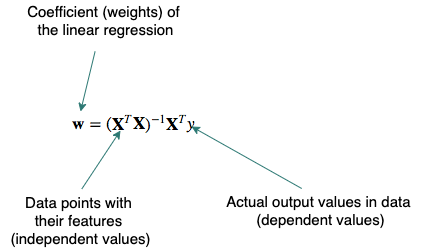
For this question, the easiest solution is to use the closed-form solution as it is easy to code once the input can fit into memory. First, let us remind ourselves of the equation:
def train_linear_reg(X, y):
    weights = np.dot(np.dot(np.linalg.inv(np.dot(X.T, X)), X.T), y)
return weightsIf we assume that \(X\) is a (\(r\) x \(c\)) matrix and \(y\) is a (\(r\) x \(1\)) matrix:
Time Complexity:
- \(X^T\) will take \(O(rc)\) time [result is a (\(c\) x \(r\)) matrix]
- The multiplication of this transposed matrix with \(X\) will take \(O(rc^2)\) [result is a (\(c\) x \(c\)) matrix]
- Matrix inversion would take \(O(c^3)\) [result is a (\(c\) x \(c\)) matrix]
- \(X^T\) multiplied by \(y\) will take \(O(rc)\) time [result is a (\(c\) x \(1\)) matrix]
- The final multiplication of (\(c\) x \(c\)) by (\(c\) x \(1\)) will take \(O(c^2)\) [result is a(\(c\) x \(1\)) matrix]
- Thus the time complexity is \(O(rc + rc^2+c^3+rc+c^2)\) we can reduce to \(O(rc+ c^3)\)
Space Complexity: \(X^T\) will have a space complexity of O(c²) and \(X\) has a space complexity of \(O(rc)\). Thus, the final space complexity is \(O(rc+ c^2)\).
Follow Up 1: Can you solve this with gradient descent instead?
More than likely the interviewer would like you to end up coding the gradient descent approach. So in this follow up question we would code it. Note: if the candidate first tried to code the gradient descent approach the interviewer might ask if they can code the closed form equation.
def train_linear_reg_gd(X, y, learning_rate=0.001, max_epochs=1000):
    num_datapoints, num_features = X.shape

    # set weights and bias to 0
    weights = np.zeros(shape=(num_features, 1))
    bias = 0

    for i in range(max_epochs):
        # Calculate simple linear combination y = mx + c or y = X * w + b
        y_predict = np.dot(X, weights) + bias  # O(r*c)
        # Use mean squared error to calculate the loss and then
        # get the average over all datapoints to get the cost
        cost = (1 / num_datapoints) * np.sum((y_predict - y) ** 2)  # O(r)

        # Calculate gradients
        # 1st - gradient with respect to weights
        grad_weights = (1 / num_datapoints) * np.dot(X.T, (y_predict - y))  # O(c⋅r)
        # 2st - gradient with respect to bias
        grad_bias = (1 / num_datapoints) * np.sum((y_predict - y))  # O(r)

        # update weights and bias
        weights -= learning_rate * grad_weights
        bias -= learning_rate * grad_bias

    return weights, bias
Time Complexity: Assume e is the maximum epochs. The largest inner for loop time complexity is \(O(rc)\) and we do this \(e\) times so the time complexity is \(O(erc)\)
Space Complexity: We created weights which have a space complexity of \(O(c)\). Then we produce y_predict which has a space complexity of \(O(r)\) and grad_weights with \(O(c)\). Thus, the final space complexity is \(O(2c+r)\).